Part 1 GPA Chart

ABC GPA Part 2

G.P.A. Part 1
If you are using Excel start with #1		If you are using Google Sheets start with #2.

ABC

Step by Step Instruction Google Sheets start with Step # 2
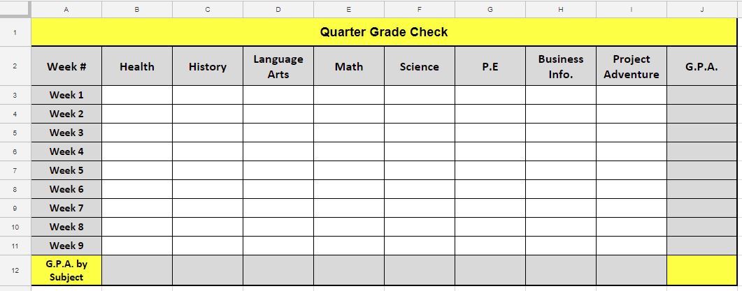
Part 1 Formatting the Google Sheet starts with # 2
1a	1b	1c	2	2a	2b	2c	2d	2e	3
Formulas
		4	5	6	7	8	GPA Part 2

Step 2.

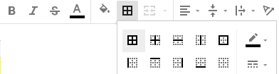
Study the Tool Bars>>>>

Google Sheets Tool Bar

Google Sheets Tool Bar

Google Sheets Tool Bar

Format the Chart

Step 2. But the Borders in.
Click to see an example.

Select cells A1- J12 and choose all borders

Step 2a) In cell A1 type the title "Quarter Grade Chart."
Step 2a-1) Merge cells > A1 - J1.

Step 2a-2) Center cells > A1 - J12.

Step 2a-3) Float titles in cells > A1 - J12.

Step 2b) In cells B2 - J2 TYPE your Class Schedule.

Click the Text Wrap Tool so that Language Arts fits in the cell.

Step 2c) In cells A3-A11 Type the week number.

Type 3 Week titles and then "skinny plus" them down to cell A11.

Step 2d) In cells A12 type the title "G.P.A. by Subject."

Click the Text Wrap Tool so that "G.P.A. by Subject" fits in the cell.

Step 2e)

Type the number four in Cell G6.

Type the number three in Cell E4.

Type the number two in Cell B7.

Type the number one in Cell H9.

Type the number zero in Cell E5.

Step 3

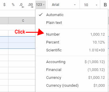
Number Format

Step 3a) Complete Step 2e) by typing a few G.P.A. numbers into the chart. 4's, 3's, 2's, 1's or 0's.

Step 3b) Now select cells B3 - J12.

Step 3c) Set the Number Value.


Step 3d) Set the decimal value
                                   to round to the nearest tenths position.
                             From a 3 to a 3.00 to a 3.0
                             From a 2 to a 2.00 to a 2.0
                             From a 1 to a 1.0 to a 1.0 etc.

Google Sheets ChooseNumber Tool Bar

Change to Number

Step 4

Imput Formulas

Google Sheets Formula Tool Bar

Step 4. In Cell J3 type in the = Average Formula:

=AVERAGE(B3:I3) Press Enter

Use the "skinny plus +" to extend the Average Formula all the way down the column J.

Select Cell J3 > Move your mouse around until it changes to a "skinny plus." >
Click > Hold > Drag down the column > until you reach J11 > Release.

When you have an AVERAGE Formula in a cell but there are
no numbers in the cells you'll get the Error Message .

We'll get rid of the Error Message in Step 8.

Step 5

Step 5. In Cell B12 type in the = Average Formula:

=AVERAGE(B3:B11) Press Enter

Use the "skinny plus +" to extend the Average Formula to the right for the entire row.

Select Cell B12 > Move your mouse around until it changes to a "skinny plus." >
Click > Hold >Drag to the left >until you reach J12 > Release.

Step 6

Error Messages

Watch the video

or
follow the
Step by Step
Instructions.

When you have an AVERAGE Formula in a cell but there are
no numbers in the cells you'll get the Error Message

Step 6. Let's Hide the Error Message

How to get rid of the Error Messages

3:05 min

Step 6 - Let's Hide the Error Message

Step by Step Instructions

Step 6a Select Cell J3 that has the

Error Message.

Step 6b Edit the Average Formula =AVERAGE(B3:I3)


Step 6c	Put your cursor between the = sign and the A in average.
Step 6d	Type iferror(
Step 6e	Put your cursor behind the last )
Step 6f	Type a comma , 2 quotes "" and a )

Step 6g) Your "If Error Formula" should look like this:

Step 6h) Use the "skinny plus +" to extend the NEW Formula all the way down the column.

Select Cell J3 > Move your mouse around until it changes to a "skinny plus." >
Click > Hold > Drag down the column > until you reach J11 > Release.

Step 7

Step 7 Repeat the Steps from 6 in Row 12 but use (B3:B11)

Step 7a Select Cell B12 that has the Error Message.

Step 7b Edit the Average Formula so that it looks like the "If Error Formula" below.

Step 7c Use the "skinny plus +" to extend the NEW Formula all the way to the left of the row.

Select Cell B12 > Move your mouse around until it changes to a "skinny plus." >
Click > Hold >Drag to the left >until you reach J12 > Release.

Step 8 Get your Grade Report from Ms. Church and input your Quarter Grades.

Tell Ms. Church that you are ready for Part 1 to be graded.

GPA Chart Part 2

	Frequently Asked Questions
	UP

	Where is the AUTO SUM button? a.k.a. Where is the FX button?
	UP
	Where is the Chart Button?

	UP

	Frequently Asked Questions
	UP
	Where is the FX button?

	UP

	Frequently Asked Questions
	UP
	Where is the Chart Button?

	UP

	Frequently Asked Questions
	UP
	Where is the Text Wrap Button?	Where is the Merge and CenterButton?

	UP

	Frequently Asked Questions
	UP
	Where is the Settings and Print Preview? Special Note - This version there is no Print Preview Settings.
	UP
	Where is the Merge Button?
	UP
	Where is the Conditional Formatting Button?
	Ms. Church show me how to Conditional Format cells.
UP

	Frequently Asked Questions
	UP
	Where is the Chart Button?
UP

G.P.A.	Frequently Asked Questions
	Back to Video GPA
	Where is the Merge and Conditional Formatting Button?
Back to Video GPA

Just for fun Hour of Code
Sign Up	Email first name dot last name at g dot kpbsd dot org shell.church@g.kpbsd.org

G.P.A. Video

Conditional Formating Videos

Fri.	G.P.A. Video
	Create a new GPA Excel Document with drop down windows, Value Look up formulas and conditional formatting. for each G.P.A. range. Save it as LastName_FirstName_gpa
	G.P.A. Video	Conditional Formating Videos

1- Excel Video Doc
ABC	Fred's Part 1				Fred's Part 2
01	02	03	04	05	06	07	08
Drop	Drop 02-05				Drop 06-08

Part 1 Formatting the Chart in an Excel Document	Step # 1a Column Width & Row Height
	Step # 1b Format All Cells
	Step # 1c Center Alignment &Text Wrap
Formatting the Chart in Google Sheets	Step # 2 Type in your Class Schedule Google Sheets Center Alignment &Text Wrap
Number Values	Step # 3 Round to the nearest tenths. 2 should read as 2.0. 1.3333 should read as 1.0. 0.5147 should read as 0.6.
Insert Formulas	Step # 4 Average Formula in column J Put the AVERAGE formula into Cell J3 =AVERAGE(B3:I3) Then get the "skinny +" and spread the formula down Column J.
Insert Formulas	Step # 5 Average Formula in row 12 Put the AVERAGE formula into Cell B12 =AVERAGE(B3:B11) Then get the "skinny +" and spread the formula to the right of row 12.
Get rid of the Error Message	Step # 6 If Error Formula in Cells B3:I3
Get rid of the Error Message	Step # 7 If Error Formula in Cells B3:B11
Gett your Grade Check Sheet.	Step # 8 Input QUARTER grades
Tell Ms. Church that you're ready for Part 1 to be graded. Do not go on to Part 2 until you have a grade in PowerSchool.
GPA Part 2

Step by Step Instruction Google Sheets start with Step # 2
Part 1 Formatting the Google Sheet starts with # 2
1a	1b	1c	2	2a	2b	2c	2d	2e	3
Formulas
		4	5	6	7	8	GPA Part 2

Step 1

In Excel Format Cell Size

Step 1a.   In Excel Select Cells A1 - J12
          Format Cells > Column Width = 15
          Format Cells > Row height = 35-40

Step 1b. In Excel Select the Whole chart

	Format > All Borders
	Format > Bold Font
	Format > Font Calibri
	Format > Font Size 16

Step 1c. Alignment
In Excel Select the Whole chart > Wrap Text >

Next Step #2

Step by Step Instruction Google Sheets starts on Step 2
Part 1	1a	1b	1c	2	2a	2b		2c	2d	2e	3
4	5	6	7	8	Part 2		9	10	Part 3	11	12	13