Step 2

Business Info


Step 2
Format Your Sheet
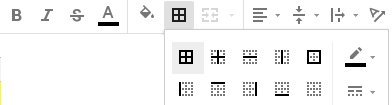
  Borders > Center > Float Cells > Text Wrap

Select cells A1- J12

Click > Hold - Drag to Select cells A1 - J12 > Choose All Borders .

Select cells A1- J12

Click > Hold - Drag to Select cells A1 - J12 > Choose Center

               Click on the shark's tooth then click Center.

Select cells A1- J12

Click > Hold - Drag to Select cells A1 - J12 > Choose Float Cells

in the center of the cell > c
lick on the shark's tooth then click Middle Align.

Select cells A1- J12

Click > Hold - Drag to Select cells A1 - J12 > ChooseText Wrap

The
titles will fit into the cells. Click on the shark's tooth then click Text Wrap.

Step 2a

Format Your Sheet - Chart Title

Step 2a) In cell A1 type the title " Quarter G.P.A. Chart "    


Step 2a-1 Format Your Sheet - Merge then click Center

Step 2a-1)      Merge cells > A1 - J1.

Click >Hold > Drag to Select cells A1 - J1 >
Merge All > Center


Step 2a

Format Your Sheet - Type Your Schedule.

Step 2a) In cell A1 type the title Quarter G.P.A. Chart

Starting in A2 type Week #

Then in B2 type in your current class schedule in order from
                                                Period 1-7, Include your Advisory, and then type G.P.A. in Cell J2.

Week #

History     World
                or
History     U.S.

Language Arts

Math
       Algebra              or
Math
       Course 2            or
Math        Course 3

Physical Education

Science
    Life                    or
Science     Physical

Advisory

Art Introduction or Exploring Science or World Languages etc.

Business Information or Woods
or Robotics etc.

G.P.A.


Step 2c


Capitalize
the
first
letters!

Step 2c) In cells A3 - A11 Type the week numbers.

Type Week 1 in cell A3.

Type Week 2 in cell A4.    

Type Week 3 in cell A5.


Move the cursor from a "fat plus"
             to a "skinny plus" then Click > Hold > Drag down to cell A11.

This will copy the Week #'s into the rows.


Step 3 Format the Numbers

Step 2e

Format the Chart - Type numbers into the chart.

Step 2e)

Type a number 4 in Cell G6.

Type a number 3 in Cell E4.

Type a number 2 in Cell C7.

Type a number 1 in Cell H9.

Type a number 0 in Cell E5.


Step 3 Format the Numbers