Step 12 Google Sheets - The 4th Quarter has 10 weeks     Insert a row above Row A12 so you may include the 10th week that is in the 4th quarter.
	Click for the Excel Instructions.
INSERT ROW 12a. Select the 4th Quarter Grade Check Chart. 12b. Select Cell A 11 > Right Click > Insert Row           This will add a row between Week 8 and Week 9. 12c. Type a 4 in cell B 12.       You'll see that the                    Conditional Formatting also works.      In cell B 13 your formula has adjusted to include the new row. See the example to the right..
12d. Title the row correctly. "Week 10 grades" Select cell A 10 "Week 8" > Move your mouse around                 until it changes to a "skinny plus." > Click> Hold >Drag down to Cell A 12.                 Your Week titles will change automatically.
Click here if your formulas do not work or if you're using Excel for your charts.

 

 

 

 

 

 

 

 

 

 

 

 

 

 

 

 

 

 

 

 

 

 

 

 

 

 

 

 

 

 

 

 

 

 

 

 

 

 

 

 

 

 

 

 

 

 

 

 

 

 

 

 

 

 

 

 

 

 

 

 

 

 

 

 

 

 

 

 

 

 

 

 

 

 

 

 

 

 

 

 

 

 

 

 

 

 

 

 

 

 

 

 

 

EXCEL Edit ALL Formulas to include Row 12. Step by Step to....

Edit the formula to include the new row.

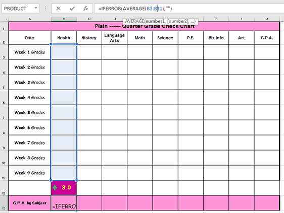
1. Put a Number in Cell B12 then Click on cell B13.

2. See below for the example.         Put your cursor in the B3:B11 area of the formula.         Once you click the Column will be highlighted.

3. Now drag down the "Skinny Blue +" to include the cell in your formula.

4. Press Enter

5. Click Hold Drag the "Skinny Green +"in Cell J13 to the left         to copy the formula into the other cells in the row.

6. Press Enter

7. Repeat Steps 1-5 for Cell J3 and the rest of Column J

5. Edit ALL Conditional Formatting to include Row 12.