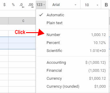
Format Numbers to appear a decimal.

If you skipped step Step2e)
Step 3a)   Type a few G.P.A. numbers into the chart. 

4

3

2

1

0

Step 3b) Now select cells B3 - J12.  
     
Step 3c) Set the Number Value.

                                      

                                              

Step 3d) Set the decimal value to automatically
                                    round to the nearest tenths position.

Click this until your numbers look like:
                         

4.00   Click        4.0

 

Now when you type a

4      3       2      1      or      0

it will automatically type in a

4.0      3.0       2.0      1.0      or      0.0