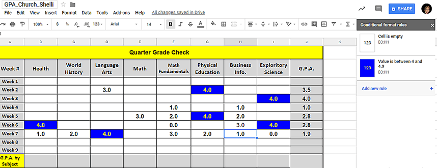
Table of Contents for Part 2

Business Info

Part 3

Step 9.

Conditionally
Format
the cells to
change colors
with every
G.P.A.

9a.    
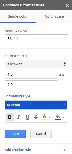
Now add another rule for each GPA number and format the rule.
After you typw the rule a number will change to the color that you choose.

Make sure that cells B3 - I11 are still selected.
                 Format   >  Conditional Formatting   >   Add New Rule


   >   
Arrow up to the Excel Table


9b. Change the rule from "is empty"   to "is between."

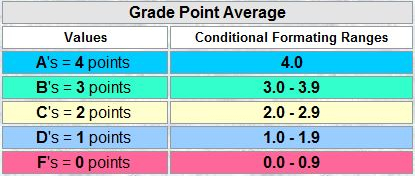
9c. Make every G.P.A. range a different color.

Grade Point Averages
Values
Format cells if ...
Ranges
F's = 0 points
is between.
0.0 - 0.9
D's = 1 points
1.0 - 1.9
C's = 2 points
2.0 - 2.9
B's = 3 points
3.0 - 3.9
A's = 4 points
4.0 - 4.9
extra credit

9d. Select a new color and text color for each GPA range.
                   
      
 If you go with a dark color background choose a light color text.
                          
If you go with a light color back ground choose a dark color text.

Repeat for each GPA Range.

Arrow up to the Excel Table

Table of Contents for Part 2


pg


pg


pg


pg


pg


pg


pg


pg


pg


pg


pg


pg


pg


pg


pg


pg


Arrow up to the Excel Table


Excel
Step 9.

Is Blank Rule


Watch the video


Change the cell color of Blank Cells to White.
2:24 mi


Excel gives Blanks cells a zero value, therefore,
you need to add an Is Blank formula so that the cell that
Is Blank will be white.


Ms. Church show me how to change the chart from pink to white.
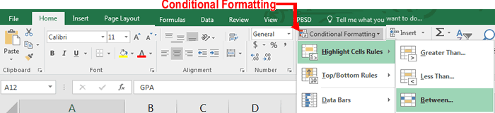
IS BLANK Video


Conditional Formatting In EXCEL

Arrow up to the Excel Table

Excel

Step 10

Conditional Formatting

Watch the video
Ms Church show me how....
or
follow the
Step by Step
Instructions.


Arrow up to the Excel Table


Step 10)   

Select the whole chart and input the
Conditional Formating
for the GPA Ranges.
                      

Ms. Church show me how to Conditionally Format cells.

Ms Church show me how....

One more step in Part 2 to complete.
Scroll down to Step 10.
Arrow up to the Excel Table


pg


pg


.